Economic 101
Many different disciplines (e.g. Game Theory, Sociology, Psychology, Political science, …) can shed some light on strategic management. This section briefly explores how micro-economics can help clarify some key concepts of strategy, particularly in the perspective of value architectures.
The environment (society, competitors, infrastructure, regulation, government) influences the type of strategy that firms can form. Still some firms will choose appropriate strategies and succeed while other will fail.
„Successful strategy result from applying consistent principles to constantly changing business conditions. Strategies are the adaptive and principled responses of firms to their surroundings. ” [D. Besanko]
Remember, this is only a brief introduction. The interested reader should turn to reference books such as (( [Besanko13] [Pindyck12] [Mas-Colell95] [Varian14] ) )
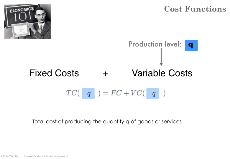
TOTAL COSTS, FIXED COSTS, VARIABLE COSTS
The total cost \( TC \) of producing a quantity \( q \) (considered as a flow i.e. production of a certain quantity in a given period of time – usually a year or a month) is the sum of fixed costs \( FC \) which don’t depend on \( q \) and variable costs \( VC \) which is a function of \( q \).
\[ TC(q) = FC + VC(q) \]
Note: \(VC(q)\) is the cost of producing \(q\) units (and not the unitary cost when the level of production is \(q\).
It is noteworthy that the notion of fixed vs variable depends on the considered time horizon. In the very short term most costs are fixed (as a firm can usually not react instantaneously to changes) and by contrast in the very long run all costs are variable (a firm may decide to sell existing fixed assets or on the contrary to acquire additional ones). Usually we consider that i) a firm commits to a production technology, tooling and facilities (fixed costs) with a maximum output level and ii) the firm can adjust its production level (variable costs) within these boundaries.
Selecting a technology induces a total cost function. Two different technologies (i.e. two different ways to produce the same outputs) will usually have different fixed and variable costs.
Selecting a production level determines the average cost. For a given production level, the notion of average costs helps comparing the two.
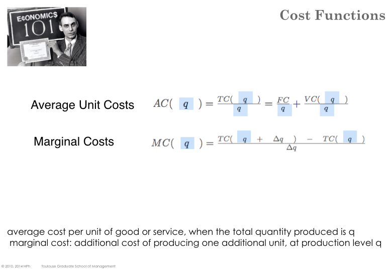
AVERAGE COSTS
The average cost \( AC \) is the total cost (at a given level of production) divided by the quantity produced.
\[ AC(q) = \frac{TC(q)}{q} = \frac{FC + VC(q)}{q} \]
Why is this notion important? Because it provides a per-unit-cost. In other words, knowing that the production level is \( Q \), then we can consider that it costs \( n.AC(Q) \) to the firm to produce \( n \) pieces of output (don’t confuse \(n\) the number of costed units with \(Q\), the total production level ).
\( AC \) is usually not constant (i.e. it depends on \(Q\) the total quantity produced). The average cost curve is usually U-Shaped (although it can also be L-Shaped).
In many industries, the average cost tend to decrease with production volume. This is for instance, the case when fix costs are high relative to variable costs (the amortization of fix costs can be spread over more units). When the production level reaches a certain threshold, the average cost remains stable over a production range and starts to increase again above a certain level.
MARGINAL COSTS
The marginal cost (at a given production level) is the incremental cost of producing one additional unit.
\[ MC(q) = \frac{TC(q + \Delta q) - TC(q) }{ \Delta(q)} = - \frac{FC + VC(q +\Delta q) - FC - VC(q) )}{\Delta q} = \frac{ VC(q +\Delta q) - VC(q) )}{\Delta q}\]
In other words, \( MC \) is the derivative of \( TC \) as well as \( VC \) (\( FC \) being a constant, its derivative is null).
\[ MC(q) = \frac{d TC(q)}{dq} = \frac{d VC(q) }{ dq} \]
The derivative of the Average cost is
\[ \frac{dAC(q)}{dq} = -\frac{F+VC(q)}{q^2} + \frac{1}{q}.\frac{dV(q)}{dq} \] which can be rewritten:
\[ \frac{dAC(q)}{dq} = \frac{1}{q} (\frac{dV(q)}{dq} -AC(q)) = \frac{MC(q) - AC(q) }{q} \]
When the marginal costs is lower than the average cost, the average cost curve is decreasing. When the marginal cost equals the average cost the average cost curve is flat (and at its lowest value) and when the marginal cost is higher than the average cost, the curve is increasing.
The optimum corresponds to \( AC(q) = MC(q) \).
SUNK COSTS, AVOIDABLE COSTS
One of the key principle of micro-economics is that when a firm is facing a decision, past decisions cannot be undone and only that costs that the decision affects should be considered.
Sunk costs are those costs that are already incurred and cannot be recovered (not matter what). Once incurred they should be ignored in any future decision. Avoidable costs are those costs that can be recovered.
Ignoring sunk costs leads to a frequent fallacy. Assume that you launch the development of a product under the assumptions that it will cost 10 million. As you have already spent 8 million, a direct competitor unveils a similar product which cuts your addressable market by two. The 8 million already spent are sunk costs (assuming that what has been done cannot be re-used for any other purpose). So the decision to continue or stop should only be based on comparing the new market perspective with the 2 million investment that are still required to complete the development (and not the initial 10).
It is important to recognize that not all fixed costs are sunk costs. If you acquire an office building to host your headquarters you always have the option to re-sell it later (not necessarily at the same price though). By contrast, if you build rail tracks between two of your factories, it is very likely that associated investment are sunk costs.
Identifying Sunk costs is key to understand the structure of an industry and entry / exit decisions.More globally it is highly advisable to recognize before committing to any large expense what will be sunk cost and what will be avoidable cost.
ECONOMIC vs ACCOUNTING COSTS
Accounting tend to recognize three main types of costs: direct costs (aka Cost of Good Sold), indirect costs (aka Sales, General Management & Administration) and Amortization & Depreciation.
Accounting statements such as the balance sheet and income statement are aimed at external audience (tax authorities, lenders, shareholders & investors). Accounting numbers are based on historical costs. For instance, to assess the value of an inventory of raw material, accounting will consider the (weighted average) price at which it has been purchased.
Business decisions (starting with strategy related decisions) however should be based on economic costs (aka opportunity cost). In the example above, the value of an inventory is the price at which it could be sold on the market (regardless of the price at which it had been purchased by the firm).
We will see in the Value Equation section that to attract investors, a firm must generate a return that is at least as large as the return they could have received from the best investment of similar risk.
Price elasticity of demand
According to the law of demand (one of the most fundamental principle in micro-economics) the overall quantity of a good that consumers are ready to buy is a function of the price of the good. The higher the price the less quantity is sold.
When a firm changes its pricing policy (for instance increases the price) it will impact its addressable market (for instance sell less), its average cost and its profit. While this principle applies to all industries the magnitude of the effect is highly variable from one good to the next (and depends usually as well on the level output).
The elasticity of demand measures the sensitivity of the effect. It is defined as the variation of demand relatively to the variation of price.
\[ \epsilon = - \frac{\frac{dq}{q}}{\frac{dP(q)}{P(q)}}\]
If \( \epsilon \) is less than 1, the demand is inelastic. A classical example is fuel (gasoline) with elasticity around 0.1 to 0.2 - which means that even when fuel price double, the total quantity is reduced by around 30%. At the extreme when \( \epsilon \) is null, the demand is totally inelastic (the quantity sold remains identical no matter the price level).
If \( \epsilon \) is more than 1, the demand is elastic.
Price elasticity can be assessed numerically (that typically what econometrics an do). Qualitatively a product is more price-sensitive (elastic) when i) differentiation compared is limited and competitors’ price are easily accessible, ii) the price of the product represents a large chunk of the buyer’s expenditure or budget. Conversely a product is less elastic when i) comparison among competing or substitute products is difficult or costly, ii) switching costs are high, iii) the product is a complement to an other product that has very high switching costs.
In a highly competitive market, if one firm only changes their price (and their rivals don’t match that new price) then it is likely that most of the demand will shift to the firms with the lowest price.
In a situation of perfect competition, a firm has no impact on the market price (firms are price takers) and the demand curve that see each firm is constant (an horizontal line at the market price \( P = P^* \)). In that case price elasticity is infinite.
TOTAL and MARGINAL REVENUE
The total revenue function of a firm denotes the revenue captured by the firm as a function of its level of production \( q \). The total revenue equals the quantity times the price for that quantity (demand curve).
\[R(q) = P(q) * q \]
The marginal revenue is the derivative of the total revenue function and represent the addition revenue derived from selling one additional unit.
\[ \frac{dR(q)}{dq} = \frac{dP(q)}{dq} * q + P(q) = P(q) * [ \frac{dP(q)}{P}* \frac{q}{dq} + 1 ] \] \[ \frac{dR(q)}{dq} = P(q) * ( 1 - \frac{1}{\epsilon} ) \]
It follows that if demand is inelastic, ( i.e \( \epsilon \) is less than 1) then \( \frac{1}{\epsilon} \) is more than 1, which entails that \( ( 1 - \frac{1}{\epsilon} ) \) is negative and therefore the total revenue decreases.