Horizontal Boundaries
The Horizontal boundaries correspond to the quantity (and variety) of product sold by a single firm. The horizontal boundaries can be measured in market share. Economies of scale, scope and experience allow some firm to derive of cost advantage that can translate either in lower price or higher profit.
Horizontal boundaries must be understood within a segment of the Value system (i.e. within one given industry). It mainly relates to the size of a company and how much market share it controls.
A firm can expand its horizontal boundaries through organic growth (increasing its production level / sales) or through acquisition of firms operating in the same industry. The principal benefit of engaging in horizontal integration is that i) it eliminates competition from other firms and ii) it allows to increase economies of scale (when applicable) and reduce the average unit costs.
As vertical and horizontal integrations can significantly modify the market power of firms, they are under the scrutiny of governments and antitrust authorities.
Economies of SCALE & SCOPE
“Informally when there are economies of scale and scope bigger is better” [Besanko]”
Definition of Scale economy
In many industries, average unit costs tend to decrease with the production volume (at least until a certain production threshold). This is for instance the case when the fixed costs are high relative to variable costs (the amortization of fixed costs can be spread over more units).
„The production process for a specific good or service exhibits economies of scale over a range of output when average cost (i.e. cost per unit of output) declines over that range. Economies of scale refer to the advantages that flow from producing a larger output at a given point in time: i.e. the ability to perform an activity at a lower unit cost when it is performed on a larger scale at a particular point in time. ” [D. Besanko]
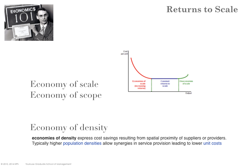
The area where marginal costs (the incremental costs of producing one more item) are less than average costs brings up economies of scale (aka increasing returns). A firm has a strong incentive to increase its production level within the area of increasing returns (the higher the production level, the lower the unit costs).
The smallest quantity for which economies of scale are exhausted (i.e. where the constant return area starts ) is named the minimum efficient scale
However, if the firm continues to increase its production level, sooner or later it will hit the area of decreasing returns and starts to generate diseconomies of scale (for instance because the new production level would require an additional facility which would increase fix costs).
Multi-business firms may enjoy economies of scope when some inputs (procured parts, production activities) are used for several pro- ducts. In such a case the cumulated production (of all such products) is taken into account to compute unit costs (average total cost per unit). The existence of economies of scope between two different businesses may underpin some corporate advantage. Owning the two businesses creates value in addition to the intrinsic value of each business taken in isolation.
When an average cost curve is L-shaped, costs decrease up to the minimum efficient scale of production and remain stable beyond.
Examples
Example with linear variable costs
Let’s assume that the variable cost is a linear function, i.e. \( VC(q) = a.q \).
The total cost is \( TC(q) = FC + a.q \) and the average cost is \( AC(q) = \frac{FC}{q} + a \).
The bigger the quantity \( q \) produced, the smaller the average cost (for an infinite quantity \( AC(q) \approx a\))
In that case, the marginal cost is constant \( MC(q) = \frac{VC(q)}{q} = a \) and the average cost is always decreasing. The average costs decreases when q increases as the fix part becomes more and more diluted.
Example with more complex variable costs
This time let’s assume that the variable cost is a more complex function \( VC(q) = a.q + b.q^2 \). There is still a linear part but also a quadratic element \( bq^2\)).
The total cost is \( TC(q) = FC + a.q + b.q^2 \) and the average cost is \( AC(q) = \frac{FC}{q} + a + b.q \). The marginal cost is \( MC(q) = a + 2b. q \).
The optimum corresponds to:
\( AC(q) = MC(q) \)
i.e. \( \frac{FC}{q} + a + b.q = a + 2b.q\)
i.e. \( \frac{FC}{q} = b.q\)
i.e. \( q_0 = \sqrt{\frac{FC}{b}}\)
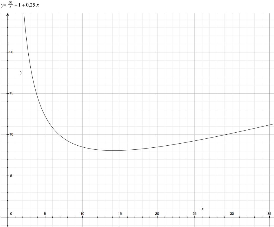
The average cost decreases until the quantity reaches \( q_0 \) and then starts to grow.
Reasons for economies of scale:
Spreading of fixed costs fixed costs derive from factors cannot be scaled down below a certain size (e.g. factories, machine). Fixed-costs also include Advertising, Research & Development costs and set-up costs (i.e. expenditures before any revenues). In many production processes, production capacity is proportional to the volume whereas total cost is proportional to the surface area.
Economies of density arise when the number of customers increase in a geographic area. Economies of density also applies to all kind of network (telecommunication, airline hub, digital platform).
Purchasing Power most suppliers give discounts based on quantities purchased
Inventories firms carry inventory to mitigate the risk of production disruption (e.g. despite a machine being out of service, the full process must continue to run while the machine is being repaired). The higher the production level, the lower the ratio of inventory (law of big numbers).
Reasons for diseconomies of scale:
Increasing production (aka production rate) usually is not without problem. As the machines are more loaded they are more prone to failures which disrupts production and entails additional costs (non quality, scrapping, additional lead time, …). More workers also means that more people are needed to coordinate, plan and lead (i.e. additional overhead, bureaucracy costs).
When production continues to grow, the fixed assets (e.g. machinery, plants, warehouses, …) will reach their limit. Increasing any further production will require increasing capacity and therefore fixed costs.
Labor Cost usually grows with larger firms as they usually offer higher compensation and benefits (wages, bonuses, work council). However it is noteworthy that worker turnover is often lower at larger firms (which reduces the one-off costs of hiring and training new recruits).
Economies of SCOPE
„Economies of scope exist if the firm achieves savings as it increases the variety of goods and services it produces” [D. Besanko]
\( TC(Q_x, Q_y) < TC(Q_x,0) + TC(0, Q_y) \)
The total cost of producing simultaneously \( X \) and \( Y \) is less than the cumulative cost of producing the two procuts separately.
EXPERIENCE CURVE
In many industries, significant productivity efficiency and improvement are gained with the cumulated level of production. Please note that economies of scale are driven by the level of production within a period (typically the year) whereas the experience effect is linked to the cumulated production level (independently of any time reference).
Learning Curve Definition
„ The learning curve (or experience curve) refers to advantages that flow from accumulating experience and know-how overtime: the reduction in unit costs due to accumulating experience over time, independently of the current scale of operation.” [D. Besanko]
The effect experience can be due to several factors:
Labour efficiency (learning by doing, getting more confident, etc)
Standardization, method & process improvement
Better automation, product redesign
In industries where the experience effect is important (for a typical firm, doubling cumulative output reduces average costs by 20%), players will seek to reach the highest cumulated production as quick as they can. They will therefore try to extend their market shares. A firm that can significantly benefit from learning, will often ramp-up production faster to gain from experience quicker.
When growth is limited, the industry structure becomes rigid (zero sum games between the players). Players will therefore seek to benefit as much as they can from any market growth (e.g. acquiring new market shares) so that they are in the most favorable situation (cost-wise) when market gets rigid. This is even more crucial in industries where products are highly standardized (commoditization) where price is the only source of differentiation.
Experience effect equation
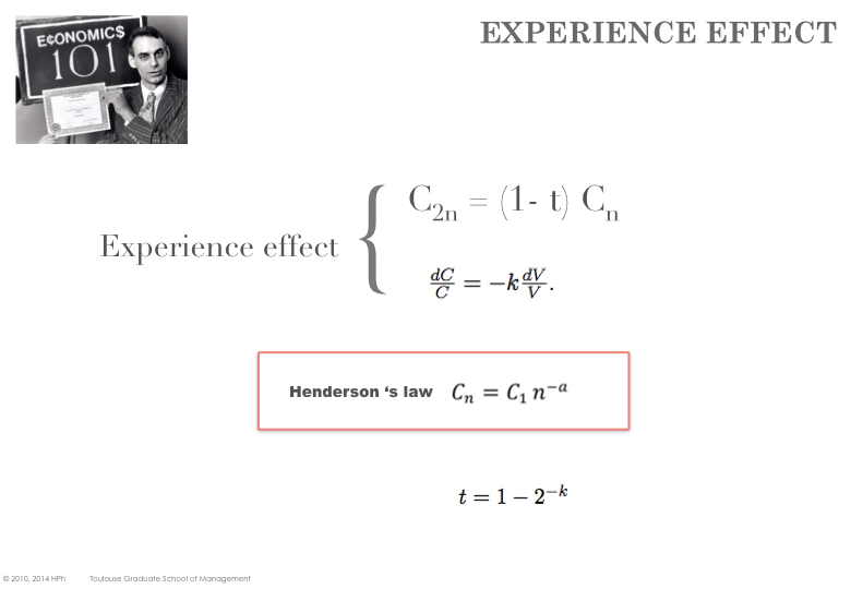
Bruce Henderson (who founded the Boston Consulting Group) had noted that the relative decrease of certain variable costs was proportional to the relative increase in cumulated production – in other words the decrease of costs in percentage is proportional to the increase in percentage of the cumulated production.
\[ \frac{\Delta C(q)}{C(q)} = -k . \frac{ \Delta q}{q} \]
This is equivalent to say that when the production doubles ( \( \Delta q = 2 q \) ), the variable cost is divided by a constant factor ( \( \Delta C(q) = -2k. C(q) \) ).
This relationship was probably first quantified in 1936 at Wright-Patterson Air Force Base in the United States, where it was determined that every time total aircraft production doubled, the required labour time decreased by 10 to 15 percent. Subsequent empirical studies from other industries have yielded different values ranging from only a couple of percentages up to 30%, but in most cases it is a constant percentage: It did not vary at different scales of operation. The Learning Curve model posits that for each doubling of the total quantity of items produced, costs decrease by a fixed proportion. [wikipedia]
The experience effect is represented by the differential equation: \( \frac{ dC(q)}{C(q)} = -k . \frac{ dq}{q} \), can be solved as \( ln(C(q)) = -kln(q) + C_0 \).
This then gives \( C(q) = \alpha . q^{-k} \).
If \( q = n \), the cost of producing the nth unit is \( C_n = \alpha . n^{-k} \).
As \( C_n = \alpha . 1^{-k} = \alpha \), then
\[ C_n = C_1 . n^{-k} \]
The unit costs of the nth unit is linked to the unit costs of the first unit. k is a constant (elasticity of costs with regard to output), specific of the industry. One can check that when the cumulated production doubles \( C_{2n} = C_1 .(2n)^{-k} = C_1n^{-k}. 2^{-k} = C_n. 2^{-k}\).
Learning curve when economies of scale are absent
When economies of scale are absent (or when a firm operate beyond the minimum efficient threshold) the average cost function is an horizontal line ( \( AC(q) = AC_1 \)). The experience effect can shit the average cost function. For instance when the cumulative production doubles then the average cost function becomes an other horizontal line ( \( AC(q) = AC_2 \) with \( AC_1 < AC_2 \) ).
Market Definition
« One cannot analyze competition without first identifying the competitors and competitors are the firms whose strategic choices directly affect one another.» ( [Besanko13] )
SSNIP
Antitrust agencies such as the DoJ (Department of Justice) in the US, the EC (European Commission) in the EU or the JFTC (Japan Fair Trade Commission)seek to limit anticompetitive conducts and to prevent situations where firms might abuse their market power.
According to the DOJ, a market is well defined and all the competitors within it are identified if a merger among them would lead to a Small but Significant (typically 5%) Non-transitory (at least for one year) Increase in Price.
Besanko provides the example of an hypothetical merger between Audi and Mercedes. Defining the market as German Luxury Cars would limit the players to Audi, Mercedes & BMW. A merger between two of these players would translate into a significant market concentration (it would reduce the number of players to 2, down from 3). However, if the market is defined as All luxury cars additional players such as Lexus, Infiniti, Jaguar should be considered as well. The SSNIP provides means to determine which market definition is the closest to reality. If by merging Audi and Mercedes could raise their prices by at least 5% then it would be the sign that they face little competition from non German brands, otherwise the larger market definition applies.